Batchelor stress tensor

In this jupyternotebook we are going to extract the local stress tensor of each individual bubble in a set of images.

# Import Libraries
import numpy as np
import matplotlib.pyplot as plt
from tifffile import imread, imsave
import skimage.measure
import pickle as pkl
import os
import spam

# Import FoamQuant library
from FoamQuant import *

# Set matplotlib default font size
plt.rc('font', size=25)

# Create the processing pipeline
ProcessPipeline = ['P5_BubbleNoEdge','Q8_Stress']

for Pi in ProcessPipeline:
    if  os.path.exists(Pi):
        print('path already exist:',Pi)
    else:
        print('Created:',Pi)
        os.mkdir(Pi)

path already exist: P5_BubbleNoEdge
path already exist: Q8_Stress

A) Type of imput data

The images we are extracting the individual bubble stress tensor are bubble-segmented images with removed labels on the edge of the images.

# Read/Save image names and directories
dirread = ProcessPipeline[0]+'/'
nameread = 'BubbleNoEdge_'
imrange = [1,2,3,4,5]

# Read the first image of the series
Lab = imread(dirread+nameread+strindex(imrange[0], 3)+'.tiff')

# Create a random colormap
rcmap = RandomCmap(5000)

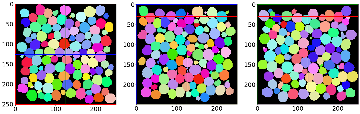
# Show a 3D-cut view of the volume
Cut3D(Lab,
      showcuts=True,
      cmap=rcmap,
      interpolation='nearest',
      figblocksize=7,           # tune this parrameter to change the figure size
      zcut=30,                  # tune this parrameter to change the orthogonal z-cut position
      ycut=False,               # tune this parrameter to change the orthogonal y-cut position
      xcut=False)               # tune this parrameter to change the orthogonal x-cut position

Number of labels: 5000

B) Quantify the individual bubble stress tensor

# Read/Save image names and directories
nameread = 'BubbleNoEdge_'
namesave = 'Batchelor_'
dirread = ProcessPipeline[0]+'/'
dirsave = ProcessPipeline[1]+'/'
# Images indexes
imrange = [1,2,3,4,5]

Batchelor_Batch(nameread,
                namesave,
                dirread,
                dirsave,
                imrange,
                verbose=True,
                endread='.tif',
                endsave='.tsv',
                n0=3)

Path exist: True

100%|██████████| 262/262 [00:23<00:00, 11.03it/s]

Batchelor_001: done

100%|██████████| 259/259 [00:23<00:00, 10.98it/s]

Batchelor_002: done

100%|██████████| 261/261 [00:23<00:00, 11.04it/s]

Batchelor_003: done

100%|██████████| 264/264 [00:23<00:00, 11.16it/s]

Batchelor_004: done

100%|██████████| 269/269 [00:24<00:00, 11.19it/s]

Batchelor_005: done

The result is for each analysed image, a .csv file, containing “number of bubble” lignes and along the columns:

• bubble label: ‘lab’

---

• bubble centroid coordinate: ‘{z,y,x}’

---

• bubble volume (vox): ‘vol’

---

• bubble area from the mesh (vox): ‘mesharea’

---

• bubble full stress tensor before dividing by the bubble volume, expressed in the basis (z,y,x):

---

• bubble full stress tensor after dividing by the bubble volume, expressed in the basis (z,y,x):

---

C) Read the results and plot the average stress field

# Read/Save image names and directories
nameread = 'Batchelor_'
dirread = ProcessPipeline[1]+'/'
# Images indexes
imrange = [1,2,3,4,5]

Llab, LCoord, Lvol,Lmesharea, LB = Read_Batchelor(nameread,
                                                  dirread,
                                                  imrange,
                                                  verbose=False,
                                                  endread='.tsv',
                                                  n0=3,
                                                  normalised=True)

Pixsize=2.48e-6 #m
SurfTens=23e-3 #N.m-1 (the surface tension)

AllB = np.concatenate(LB,0)*SurfTens/Pixsize
Bdev=[]
for i in range(len(AllB)):
    Bdev.append(SigdevfromSig(AllB[i]))
Bdev=np.asarray(Bdev)

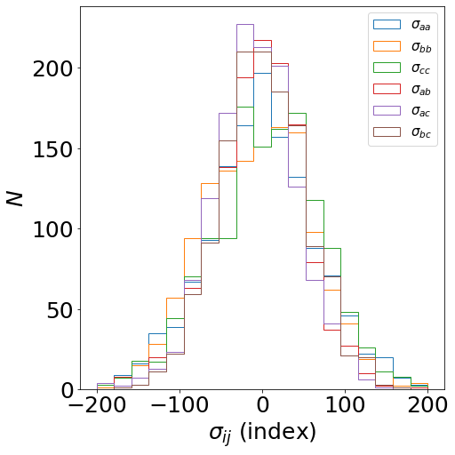
fig, C = plt.subplots(1,1, figsize = (7, 7), constrained_layout=True)

C.hist(Bdev[:,0,0], bins=np.linspace(-200,200,20), label=r'$\sigma_{aa}$', histtype='step')
C.hist(Bdev[:,1,1], bins=np.linspace(-200,200,20), label=r'$\sigma_{bb}$', histtype='step')
C.hist(Bdev[:,2,2], bins=np.linspace(-200,200,20), label=r'$\sigma_{cc}$', histtype='step')
C.hist(Bdev[:,0,1], bins=np.linspace(-200,200,20), label=r'$\sigma_{ab}$', histtype='step')
C.hist(Bdev[:,0,2], bins=np.linspace(-200,200,20), label=r'$\sigma_{ac}$', histtype='step')
C.hist(Bdev[:,1,2], bins=np.linspace(-200,200,20), label=r'$\sigma_{bc}$', histtype='step')

C.set_ylabel(r'$N$')
C.set_xlabel(r'$\sigma_{ij}$ (index)')
C.legend(fontsize=15)

<matplotlib.legend.Legend at 0x146d35db29d0>

print('Average stress, component aa', np.mean(Bdev[:,0,0]), 'Pa')
print('Average stress, component bb', np.mean(Bdev[:,1,1]), 'Pa')
print('Average stress, component cc',np.mean(Bdev[:,2,2]), 'Pa')
print('Average stress, component ab',np.mean(Bdev[:,0,1]), 'Pa')
print('Average stress, component ac',np.mean(Bdev[:,0,2]), 'Pa')
print('Average stress, component bc',np.mean(Bdev[:,1,2]), 'Pa')

Average stress, component aa -1.4105218364135446 Pa
Average stress, component bb -4.484706058504461 Pa
Average stress, component cc 5.895227894917975 Pa
Average stress, component ab -4.027057280257984 Pa
Average stress, component ac -8.993068354806914 Pa
Average stress, component bc 1.1800333523084872 Pa