Flow field & Tracking
In this tutorial you will learn to measure the flow field and track individual bubble.
The tutorial is divided in the following sections:
Import libraries
Quantification folders
Get familiar with the input data
Velocity field
Combine tracking
Tracked properties
A) Import libraries
[1]:
from FoamQuant import *
import numpy as np
import skimage as ski
import os
import matplotlib.pyplot as plt; plt.rc('font', size=20)
from tifffile import imread
from scipy import ndimage
import pickle as pkl
import pandas as pd
B) Quantification folders
[2]:
# Processing folders names
Quant_Folder = ['Q3_Bubble_Prop','Q7_Tracking']

# Create the quantification folders (where we are going to save our results)
for Pi in Quant_Folder:
    if  os.path.exists(Pi):
        print('path already exist:',Pi)
    else:
        print('Created folder:',Pi)
        os.mkdir(Pi)
path already exist: Q3_Bubble_Prop
path already exist: Q7_Tracking
C) Get familiar with the input data
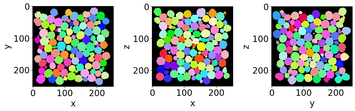
Let’s read the first bubble-segmented image of the series (with no bubble on the edges).
[3]:
# Name and directory of  the no-edge bubble segmented images
dirnoedge = 'P5_BubbleNoEdge/'
namenoedge = 'BubbleNoEdge_'

# Read the first image of the series
Lab = imread(dirnoedge+namenoedge+strindex(1, 3)+'.tiff')

# Since we are now looking at more bubbles let's create a "larger" random colormap: here 500 random colors
rcmap = RandomCmap(500, verbose=False)

# Show a 3D-cut view of the volume
Cut3D(Lab,
      nameaxes=['z','y','x'],
      cmap=rcmap,
      interpolation='nearest',
      figblocksize=4)
/gpfs/offline1/staff/tomograms/users/flosch/Rheometer_Jupyter/Jupy_FoamQuant/FoamQuant/Figure.py:90: UserWarning: The figure layout has changed to tight
  plt.tight_layout()
B) Bubble tracking
The first step when tracking the bubbles is to extract their region properties. We are going to base our tracking on the centroid and the volume of them at consecutive time steps.
[4]:
# Name and directory where we are going to save the bubble region properties
dir_Bubble_prop = 'Q3_Bubble_Prop/'
name_Bubble_prop = 'Bubble_Prop_'

# Indexes of the images of our time-series (we are working here with 10 subsequent images of the same foam sample, evolving over time).
imrange = [1,2,3,4,5,6,7,8,9,10]

RegionProp_Batch(namenoedge,
                 name_Bubble_prop,
                 dirnoedge,
                 dir_Bubble_prop,
                 imrange,
                 verbose=True,
                 endread='.tiff',
                 endsave='.tsv')
Path exist: True
Bubble_Prop_001: done
Bubble_Prop_002: done
Bubble_Prop_003: done
Bubble_Prop_004: done
Bubble_Prop_005: done
Bubble_Prop_006: done
Bubble_Prop_007: done
Bubble_Prop_008: done
Bubble_Prop_009: done
Bubble_Prop_010: done
Now that we have the bubble region properties, we can use LabelTracking_Batch to track the bubble labels between two subsequent time steps. The tracking finds the closest centroid of the bubbles in the next image. There is in addition a volume continuity criteria that allows to disregard over- or undersegmented labels. In addition, the result from discrete digital correlation can be feed-in for helping this simple tracking algorithm (not shown in this example).
[5]:
# Read/Save image names and directories
dirTrack = 'Q7_Tracking/'
nameTrack = 'Tracking'

# Tracking
LabelTracking_Batch(name_Bubble_prop,
                    nameTrack,
                    dir_Bubble_prop,
                    dirTrack,
                    imrange,
                    verbose=False,
                    endread='.tsv',
                    endsave='.tsv',
                    n0=3,
                    searchbox=[-5,5,-5,5,-5,5],   # The size of the searching box
                    Volpercent=0.05)                    # The volume continuity percentage criteria
Path exist: True
100%|██████████| 941/941 [00:00<00:00, 1108.52it/s]
Lost tracking: 87 9.24548352816153 %
100%|██████████| 938/938 [00:00<00:00, 1218.58it/s]
Lost tracking: 46 4.904051172707889 %
100%|██████████| 942/942 [00:00<00:00, 1219.16it/s]
Lost tracking: 52 5.520169851380043 %
100%|██████████| 943/943 [00:00<00:00, 1203.72it/s]
Lost tracking: 49 5.1961823966065745 %
100%|██████████| 956/956 [00:00<00:00, 1233.89it/s]
Lost tracking: 46 4.811715481171548 %
100%|██████████| 945/945 [00:00<00:00, 1239.63it/s]
Lost tracking: 36 3.8095238095238098 %
100%|██████████| 941/941 [00:00<00:00, 1222.61it/s]
Lost tracking: 16 1.7003188097768331 %
100%|██████████| 950/950 [00:00<00:00, 1232.30it/s]
Lost tracking: 36 3.7894736842105265 %
100%|██████████| 948/948 [00:00<00:00, 1158.98it/s]
Lost tracking: 29 3.059071729957806 %
Let’s open the first tracking table with pandas. It contains information about the tracked bubbles at the first time step (‘lab1’, ‘z1’, ‘y1’, ‘x1’, ‘sph1’, ‘vol1’, …) and similarly to the associated bubble at the next time step (‘lab2’, ‘z2’, ‘y2’, ‘x2’, ‘sph2’, ‘vol2’, …). It also include the displacement values from centroid to centroid (‘dz’,’dy’,’dx’).
[6]:
df = pd.read_csv(dirTrack+nameTrack+strindex(2,n0=3)+'_'+strindex(3,n0=3)+'.tsv',sep = '\t')
display(df)
| lab1 | lab2 | z1 | z2 | y1 | y2 | x1 | x2 | dz | dy | ... | sph1 | sph2 | volfit1 | volfit2 | U1 | U2 | type1 | type2 | Utype1 | Utype2 | |
|---|---|---|---|---|---|---|---|---|---|---|---|---|---|---|---|---|---|---|---|---|---|
| 0 | 1 | 6 | 15.152388 | 16.355922 | 40.837356 | 40.909404 | 84.303429 | 84.439846 | 1.203534 | 0.072047 | ... | 0.999199 | 0.999447 | 9722.445004 | 9655.570359 | 0.067219 | 0.055917 | -1 | -1 | -0.067219 | -0.055917 |
| 1 | 2 | 8 | 14.948635 | 16.062156 | 114.038778 | 114.125025 | 131.859405 | 131.406562 | 1.113521 | 0.086248 | ... | 0.998073 | 0.996529 | 9916.218343 | 10617.816823 | 0.104464 | 0.138796 | -1 | 1 | -0.104464 | 0.138796 |
| 2 | 3 | 10 | 15.792518 | 16.575670 | 199.692792 | 200.062097 | 164.094434 | 163.655742 | 0.783151 | 0.369305 | ... | 0.997768 | 0.998202 | 11081.698240 | 9876.018743 | 0.113067 | 0.101176 | -1 | -1 | -0.113067 | -0.101176 |
| 3 | 4 | 12 | 16.552135 | 17.140166 | 32.360536 | 32.686041 | 222.787112 | 222.540675 | 0.588032 | 0.325505 | ... | 0.997244 | 0.997527 | 8860.030219 | 9407.564214 | 0.125878 | 0.119138 | -1 | -1 | -0.125878 | -0.119138 |
| 4 | 5 | 13 | 16.357539 | 16.800449 | 79.266306 | 79.635258 | 184.244521 | 183.931281 | 0.442910 | 0.368953 | ... | 0.997967 | 0.997527 | 7657.430390 | 9407.564214 | 0.106439 | 0.119138 | 1 | -1 | 0.106439 | -0.119138 |
| ... | ... | ... | ... | ... | ... | ... | ... | ... | ... | ... | ... | ... | ... | ... | ... | ... | ... | ... | ... | ... | ... |
| 933 | 934 | 942 | 232.246336 | 235.004107 | 172.522232 | 171.639124 | 62.928439 | 65.383649 | 2.757771 | -0.883108 | ... | 0.998049 | 0.995721 | 8158.558661 | 10552.541454 | 0.104122 | 0.155107 | 1 | 1 | 0.104122 | 0.155107 |
| 934 | 935 | -1 | 232.539655 | -1.000000 | 231.835212 | -1.000000 | 27.378915 | -1.000000 | -233.539655 | -232.835212 | ... | -1.000000 | -1.000000 | -1.000000 | -1.000000 | -1.000000 | -1.000000 | -1 | -1 | 1.000000 | 1.000000 |
| 935 | 936 | -1 | 233.218080 | -1.000000 | 49.249668 | -1.000000 | 71.733827 | -1.000000 | -234.218080 | -50.249668 | ... | -1.000000 | -1.000000 | -1.000000 | -1.000000 | -1.000000 | -1.000000 | -1 | -1 | 1.000000 | 1.000000 |
| 936 | 937 | 939 | 232.973806 | 233.805951 | 130.775228 | 132.122098 | 169.414120 | 169.746056 | 0.832145 | 1.346871 | ... | 0.999508 | 0.998356 | 8053.805679 | 9853.325291 | 0.052833 | 0.095723 | -1 | 1 | -0.052833 | 0.095723 |
| 937 | 938 | -1 | 234.939464 | -1.000000 | 156.361704 | -1.000000 | 217.827156 | -1.000000 | -235.939464 | -157.361704 | ... | -1.000000 | -1.000000 | -1.000000 | -1.000000 | -1.000000 | -1.000000 | -1 | -1 | 1.000000 | 1.000000 |
938 rows × 28 columns
D) Velocity field
Since we have the displacement values from one image to the next, we just have to multiply by the pixel size and divide by the time-step to obtain the velocity.
[7]:
# space and time information
pizelsize = 2.75e-3 #mm
timestep = 3 #s

# The coordinates at the two time-steps
LCoord1 = np.asarray(df[['z1','y1','x1']])
LCoord2 = np.asarray(df[['z2','y2','x2']])
# Masking the data when the bubble is lost (not tracked)
mask = LCoord2[:,0] > 0

# The middle coodinates betweent the two time-steps
LCoord = (LCoord1+LCoord2)/2 * pizelsize #mm
# The velocity from the displacement field
Lv = np.asarray(df[['dz','dy','dx']])*pizelsize/timestep #mm/s
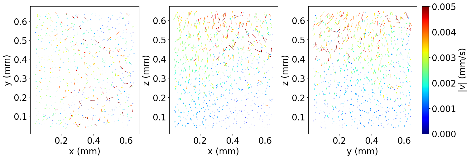
Let’s see the velocity field obtained between the two time steps. We use the function ProjVec3D for generating an orthogonal projection view (similar to Proj3D for the images).
[8]:
ProjVec3D(LCoord[mask],
          Lv[mask],
          cmap = 'jet',
          nameaxes=['z (mm)','y (mm)','x (mm)'],
          colorbarlab=r'$|v|$ (mm/s)',
          scale=0.1,
          vmin=0,
          vmax=0.005)
E) Combine tracking
We can now combine the tracking between subsequent images over the whole time series. This way, the trajectory, velocity or for exmaple bubble volume can be observed for each individual bubble over time. To do so, we use the function Combine_Tracking giving as an input the directory and name of the track tables.
[9]:
CombTrack = Combine_Tracking(nameTrack,
                            dirTrack,
                            imrange,
                            verbose=False,
                            endread='.tsv',
                            n0=3)
Some bubbles are lost and therefore not tracked over the whole time-series. The combined table is filled with ‘-1’ as soon as, at one time step, the bubble is lost. In order to plot trajectory and tracked properties figures later, we will convert all the ‘-1’ values by ‘nan’ values.
[10]:
# Convert lost bubbles data into np.nan
for axis in ['z','y','x','dz','dy','dx','rad','vol']:
    for i in range(len(CombTrack[axis])):
        for j in range(len(CombTrack[axis][i])):
            if CombTrack[axis][i][j]==-1:
                CombTrack[axis][i][j]=np.nan
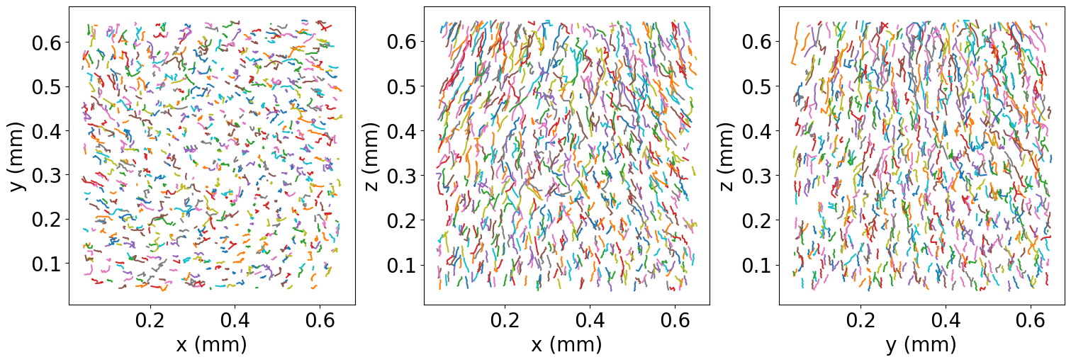
The bubble centroid coordinate is one of the tracked properties. We can observe each individual bubble trajectory as follow.
[11]:
# Show the individual paths by a random color
fig, ax = plt.subplots(1,3, figsize = (5*3, 5), constrained_layout=True)
for i in range(0,len(CombTrack['x']),1):
    ax[0].plot(CombTrack['x'][i] * pizelsize, CombTrack['y'][i] * pizelsize)
    ax[1].plot(CombTrack['x'][i] * pizelsize, CombTrack['z'][i] * pizelsize)
    ax[2].plot(CombTrack['y'][i] * pizelsize, CombTrack['z'][i] * pizelsize)
# Axes
ax[0].set_xlabel('x (mm)'); ax[0].set_ylabel('y (mm)')
ax[1].set_xlabel('x (mm)'); ax[1].set_ylabel('z (mm)')
ax[2].set_xlabel('y (mm)'); ax[2].set_ylabel('z (mm)')
[11]:
Text(0, 0.5, 'z (mm)')
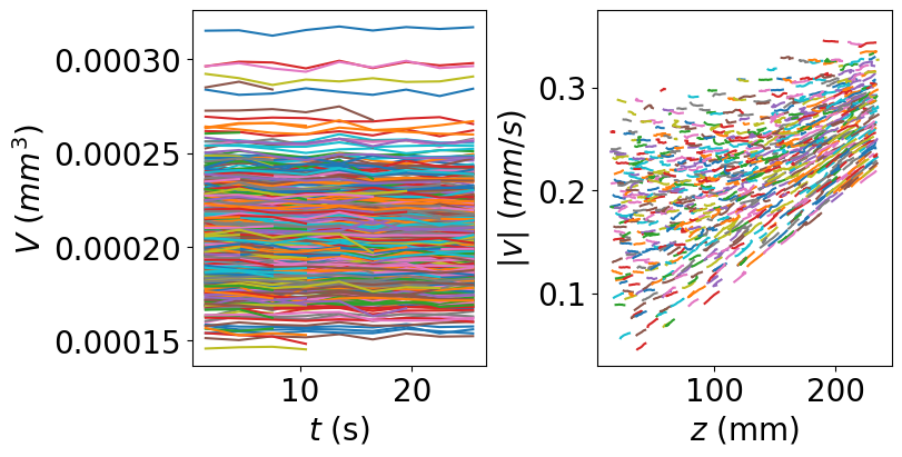
F) Tracked properties
Here is a last example of the beauty of tracking. The individual bubble volume can be observed as a function of time, and their velocity norm as a function of the vertical position in the foam (since these images originates from a flow through a hopper constriction Three-dimensional liquid foam flow through a hopper resolved by fast X-ray microtomography, it would be preferable to actually use a spherical coordinate basis, and not the cartesian (z,y,x) from our image).
[12]:
# Show the individual paths by a random color
fig, ax = plt.subplots(1,2, figsize = (4*2, 4), constrained_layout=True)

Ntstep = len(CombTrack['x'][0])
time = np.linspace(0.5,Ntstep-0.5,Ntstep) * timestep # s

for i in range(0,len(CombTrack['x']),1):

    Volume = CombTrack['vol'][i]*pizelsize
    ax[0].plot(time, CombTrack['vol'][i]*pizelsize**3)

    vz, vy, vx = CombTrack['z'][i], CombTrack['y'][i], CombTrack['x'][i]
    vnorm = np.sqrt(vx**2 + vy**2 + vz**2) *pizelsize/timestep #mm/s
    ax[1].plot(CombTrack['z'][i], vnorm)

ax[0].set_xlabel(r'$t$ (s)')
ax[0].set_ylabel(r'$V$ ($mm^3$)')

ax[1].set_xlabel(r'$z$ (mm)')
ax[1].set_ylabel(r'$|v|$ ($mm/s$)')
[12]:
Text(0, 0.5, '$|v|$ ($mm/s$)')
You have now completed this tutorial. I hope it has been helpfull to you. Go back to FoamQuant - Examples for more examples and tutorials.