Strain & Stress fields

In this tutorial you will learn to measure liquid fraction and individual bubble radius from respectively phase-segmented (cleaned) and bubble segmented (no-edge) images.

The tutorial is divided in the following sections:

• Import libraries

• Quantification folders

• Get familiar with the input data

• Strain - Shape tensor

• Strain - Texture tensor

• Stress - Batchelor tensor

A) Import libraries

from FoamQuant import *
import numpy as np
import skimage as ski
import os
import matplotlib.pyplot as plt; plt.rc('font', size=20)
from tifffile import imread
from scipy import ndimage
import pickle as pkl
import pandas as pd

B) Quantification folders

# Processing folders names
Quant_Folder = ['Q3_Bubble_Prop','Q4_Topology','Q5_Texture','Q6_Stress']

# Create the quantification folders (where we are going to save our results)
for Pi in Quant_Folder:
    if  os.path.exists(Pi):
        print('path already exist:',Pi)
    else:
        print('Created folder:',Pi)
        os.mkdir(Pi)

path already exist: Q3_Bubble_Prop
path already exist: Q4_Topology
path already exist: Q5_Texture
path already exist: Q6_Stress

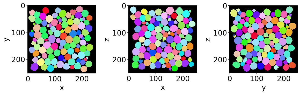
Let’s read the first bubble-segmented image of the series (with no bubble on the edges).

C) Get familiar with the input data

# Name and directory of  the no-edge bubble segmented images
dirnoedge = 'P5_BubbleNoEdge/'
namenoedge = 'BubbleNoEdge_'

# Read the first image of the series
Lab = imread(dirnoedge+namenoedge+strindex(1, 3)+'.tiff')

# Since we are now looking at more bubbles let's create a "larger" random colormap: here 500 random colors
rcmap = RandomCmap(500, verbose=False)

# Show a 3D-cut view of the volume
Cut3D(Lab,
      nameaxes=['z','y','x'],
      cmap=rcmap,
      interpolation='nearest',
      figblocksize=4)

/gpfs/offline1/staff/tomograms/users/flosch/Rheometer_Jupyter/Jupy_FoamQuant/FoamQuant/Figure.py:90: UserWarning: The figure layout has changed to tight
  plt.tight_layout()

D) Strain - Measured from the bubble region (shape tensor)

The shape strain tensor \(U_S\) is computed from the shape tensor \(S\). Each bubble is represented by a set of coordinates {\(\textbf{r}\)} of all the voxels defining its region in the image. From this set can be defined both the center of mass coordinates, \(\langle \textbf{r} \rangle\), and the shape tensor as

\(\textbf{S}=\langle(\textbf{r}-\langle \textbf{r} \rangle) \otimes (\textbf{r}-\langle \textbf{r} \rangle)\rangle^{1/2}\)

The strain tensors \(\textbf{U}_\textbf{S}\) is derived from \(\textbf{S}\) as the deviation from an isotropic shape \(\mathbf{S_0}\) state (a perfect sphere):

$:nbsphinx-math:textbf{U}_:nbsphinx-math:textbf{S} = \log`(:nbsphinx-math:textbf{S}`) - \log`(:nbsphinx-math:mathbf{S_0}`) $

with \(\mathbf{S_0} = S_0 \textbf{Id}\) and \(\textbf{Id}\) the identity tensor. The isotropic state is build from the three shape tensor eigenvalues \(\lambda_i\) as \(S_0 = (\lambda_1 \lambda_2 \lambda_3)^{1/3}\).

The shape tensor is already included in the saved properties by the RegionProp_Batch function.

# Name and directory where we are going to save the bubble region properties
dir_Bubble_prop = 'Q3_Bubble_Prop/'
name_Bubble_prop = 'Bubble_Prop_'

# Indexes of the images of our time-series (we are working here with 10 subsequent images of the same foam sample, evolving over time).
imrange = [1,2,3,4,5,6,7,8,9,10]

RegionProp_Batch(namenoedge,
                 name_Bubble_prop,
                 dirnoedge,
                 dir_Bubble_prop,
                 imrange,
                 verbose=True,
                 endread='.tiff',
                 endsave='.tsv')

Path exist: True
Bubble_Prop_001: done
Bubble_Prop_002: done
Bubble_Prop_003: done
Bubble_Prop_004: done
Bubble_Prop_005: done
Bubble_Prop_006: done
Bubble_Prop_007: done
Bubble_Prop_008: done
Bubble_Prop_009: done
Bubble_Prop_010: done

Let’s open the first saved bubble-properties table with pandas.

df = pd.read_csv(dir_Bubble_prop+name_Bubble_prop+strindex(1,n0=3)+'.tsv',sep = '\t')
display(df)

	lab	z	y	x	vol	rad	area	sph	volfit	S1	...	e2y	e2x	e3z	e3y	e3x	U1	U2	U3	U	type
0	1	15.286670	79.575571	183.687352	7622.0	12.208438	1889.990904	0.997457	7696.702997	11.356878	...	12.123131	0.558382	-0.565461	0.558382	12.288122	-0.075555	0.016856	0.058699	0.118985	1
1	2	16.593385	130.636373	17.162980	9584.0	13.177087	2204.247246	0.996115	9674.503042	12.035502	...	12.727413	-0.753596	-0.022763	-0.753596	12.968875	-0.093752	0.022430	0.071322	0.146864	1
2	3	15.635897	172.321484	101.120593	10324.0	13.507857	2309.744140	0.997574	10400.092065	12.805426	...	13.886619	-0.036291	-0.224959	-0.036291	13.241960	-0.055850	-0.019896	0.075747	0.117809	-1
3	4	15.538057	175.370390	217.745069	9328.0	13.058701	2154.914928	0.997516	9371.282698	12.381921	...	12.635434	-0.351062	0.549606	-0.351062	12.901907	-0.054760	-0.022566	0.077326	0.119294	-1
4	5	15.121800	200.194312	163.705468	10936.0	13.769663	2403.553261	0.997433	11037.743266	13.050254	...	14.409886	0.621144	-0.254747	0.621144	13.336950	-0.056747	-0.021472	0.078219	0.121240	-1
...	...	...	...	...	...	...	...	...	...	...	...	...	...	...	...	...	...	...	...	...	...
936	937	232.931714	209.884521	86.382444	9387.0	13.086175	2168.907873	0.998400	9475.291923	12.489027	...	13.894511	-0.170001	-0.174207	-0.170001	12.962521	-0.049827	-0.009192	0.059018	0.095265	-1
937	938	234.656031	34.253836	50.915761	9841.0	13.293833	2235.291662	0.997166	9895.232739	12.680207	...	12.997291	-0.130880	-0.529484	-0.130880	12.878073	-0.049090	-0.035787	0.084877	0.127836	-1
938	939	234.123875	156.617150	218.298716	9889.0	13.315411	2238.448309	0.998684	9938.866176	12.619337	...	13.528568	-0.152264	0.059711	-0.152264	13.724473	-0.055368	0.015737	0.039632	0.085592	1
939	940	234.464956	224.364352	219.393250	9274.0	13.033453	2143.488520	0.998308	9307.919924	12.256650	...	12.866831	-0.005062	0.036705	-0.005062	13.650618	-0.062668	0.017493	0.045175	0.097010	1
940	941	234.799707	24.502990	72.834127	8193.0	12.505991	1977.594288	0.999019	8257.341727	11.949345	...	12.912100	0.136215	0.314278	0.136215	12.591211	-0.048139	0.014913	0.033226	0.073929	1

941 rows × 26 columns

Let’s keep the shape tensor tensor columns

#Shape tensor
df[['e1z','e1y','e1x',
    'e2z','e2y','e2x',
    'e3z','e3y','e3x']]

	e1z	e1y	e1x	e2z	e2y	e2x	e3z	e3y	e3x
0	12.390694	0.206741	-0.565461	0.206741	12.123131	0.558382	-0.565461	0.558382	12.288122
1	14.053116	-0.391930	-0.022763	-0.391930	12.727413	-0.753596	-0.022763	-0.753596	12.968875
2	13.557547	0.846910	-0.224959	0.846910	13.886619	-0.036291	-0.224959	-0.036291	13.241960
3	13.761952	-0.256240	0.549606	-0.256240	12.635434	-0.351062	0.549606	-0.351062	12.901907
4	13.758225	-0.470152	-0.254747	-0.470152	14.409886	0.621144	-0.254747	0.621144	13.336950
...	...	...	...	...	...	...	...	...	...
936	12.564094	-0.058917	-0.174207	-0.058917	13.894511	-0.170001	-0.174207	-0.170001	12.962521
937	14.152835	0.463591	-0.529484	0.463591	12.997291	-0.130880	-0.529484	-0.130880	12.878073
938	12.792572	-0.396828	0.059711	-0.396828	13.528568	-0.152264	0.059711	-0.152264	13.724473
939	12.671146	0.502182	0.036705	0.502182	12.866831	-0.005062	0.036705	-0.005062	13.650618
940	12.135317	-0.106419	0.314278	-0.106419	12.912100	0.136215	0.314278	0.136215	12.591211

941 rows × 9 columns

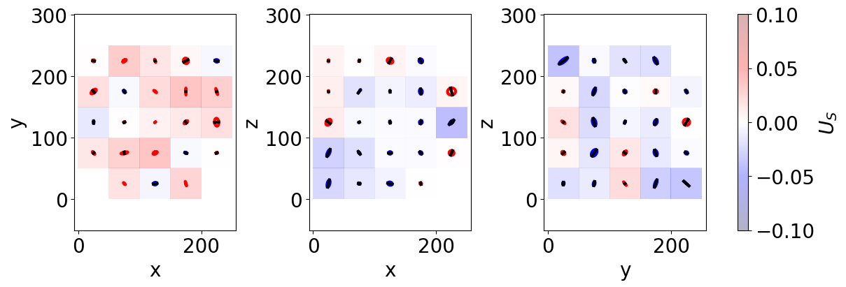
Individual bubbles are often highly deformed in what looks like random deformations. In order to extract the strain field of the structure, without this local “noize”, we spatially average the shape of the bubble inside boxes. Only after averaging, the average strain is computed from the average shape tensor.

First, let’s reshape our table in form of two lists: a list for the centroid coordinates and one for the shape tensors.

LCoord = np.asarray(df[['z','y','x']])

numpy_shape = np.asarray(df[['e1z','e1y','e1x',
                             'e2z','e2y','e2x',
                             'e3z','e3y','e3x']])
LShape=[]
for bbli in range(len(numpy_shape)):
    LShape.append(numpy_shape[bbli].reshape(3,3))

Now that we have the data in this format, one can perform a cartesian-grid average. Here we choose to have 5x5x5 boxes over the pixel coordinates [0,125] along z,y and x. We choose to return the result in a structured format.

Grids, CoordGrd, ShapeAVG, ShapeSTD, ShapeCount = Grid_Tavg(LCoord,
                                                            LShape,
                                                            Range = [0,250,0,250,0,250],
                                                            N=[5,5,5],
                                                            NanFill=True, #<- if no bubble in a box, fill with a nan value
                                                            structured=True)

# Averaged shape tensor in the fist [0,0,0] box
ShapeAVG[0][0][0]

array([[13.0621894 ,  0.35516098, -0.34083759],
       [ 0.35516098, 12.82388882,  0.36474759],
       [-0.34083759,  0.36474759, 13.22112962]])

# The associated strain tensor
USfromS(ShapeAVG[0][0][0])

array([[ 0.00213077,  0.02782792, -0.02633693],
       [ 0.02782792, -0.01634475,  0.02838876],
       [-0.02633693,  0.02838876,  0.01421397]])

To have a bit more a feeling of this strain tensor field, one can use the following representation, using ellipses. If you wish to learn about this representation, have a look at the following paper: Three-dimensional liquid foam flow through a hopper resolved by fast X-ray microtomography. CutTensor3D work similarly than Cut3D. It represents the three orthogonal cuts of the tensorial space.

CutTensor3D(Grids,
            CoordGrd,
            ShapeAVG,
            ShapeCount,
            scale_factor = 150,
            figblocksize=4,
            vmin=-0.1,
            vmax=0.1,
            Countmin=5, #<- shows a symbol if there is al least 5 bubble in the average box
            showscale=False,
            nameaxes=['z','y','x'],
            DeviatoricType=2, #<- 2 for dealing with shape: Shape -> Strain
            colorbarlab=r'$U_S$')

Normal min/max ax0 -0.014470684848635748 0.03758690547066675
Normal min/max ax1 -0.042390339076687135 0.012313103703006308
Normal min/max ax2 -0.03931547642670907 0.022374484108615564

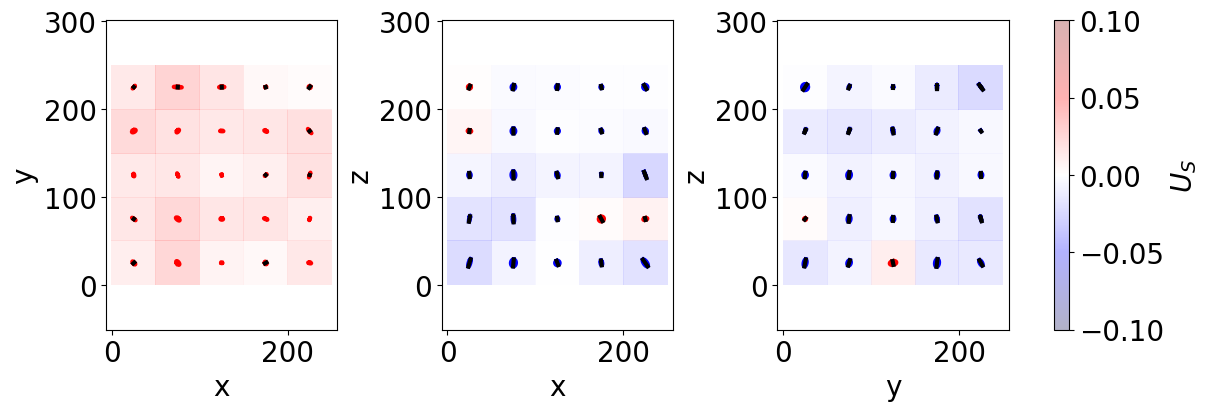
We can also do the same for the whole time-resolved data. Since we have only a small number of bubbles, it is going to smooth a bit the dentencies. In addition we can use ProjTensor3D, which average even more along the whole volume.

# Take into acount the whole time serie data
LLCoord=[]
LLShape=[]
for imi in range(len(imrange)):
    df = pd.read_csv(dir_Bubble_prop+name_Bubble_prop+strindex(imrange[imi],n0=3)+'.tsv',sep = '\t')

    LCoord = np.asarray(df[['z','y','x']])

    numpy_shape = np.asarray(df[['e1z','e1y','e1x',
                                 'e2z','e2y','e2x',
                                 'e3z','e3y','e3x']])
    LShape=[]
    for bbli in range(len(numpy_shape)):
        LShape.append(numpy_shape[bbli].reshape(3,3))

    LLCoord.append(LCoord)
    LLShape.append(LShape)

Grids_2, CoordGrd_2, ShapeAVG_2, ShapeSTD_2, ShapeCount_2 = Grid_Tavg(np.concatenate(LLCoord),
                                                            np.concatenate(LLShape),
                                                            Range = [0,250,0,250,0,250],
                                                            N=[5,5,5],
                                                            NanFill=True,
                                                            verbose=False,
                                                            structured=True)

ProjTensor3D(Grids_2,
            CoordGrd_2,
            ShapeAVG_2,
            ShapeCount_2,
            scale_factor = 150,
            figblocksize=4,
            vmin=-0.1,
            vmax=0.1,
            Countmin=5,
            showscale=False,
            nameaxes=['z','y','x'],
            DeviatoricType=2, #<- 2 for dealing with shape: Shape -> Strain
            colorbarlab=r'$U_S$')

Normal min/max ax0 0.0018644002701723728 0.02751263607400842
Normal min/max ax1 -0.025305090187731964 0.008156738035116365
Normal min/max ax2 -0.023519841267799376 0.010775489595964052

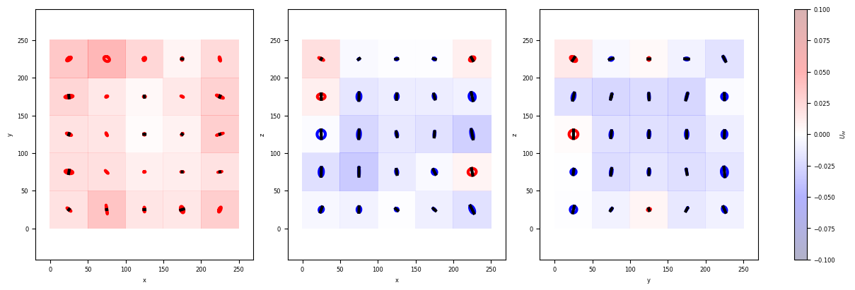
E) Strain - Measured from the distance between neighbooring bubbles (texture tensor)

We can now do the exact same steps, extracting the strain field but working with the texture tensor.

Each bubble is also characterized by a set of link vectors {\(\mathbf{l}\)} between its center and the neighboring bubble centers. The texture tensor associated to each bubble is defined as

\(\textbf{M}=\langle \mathbf{l} \otimes \mathbf{l} \rangle\)

with \(\langle ... \rangle\) the average over the set of neighboring bubbles.

The strain tensor \(\textbf{U}_\textbf{M}\) is derived from \(\textbf{M}\) as the deviation from an isotropic texture \(\mathbf{M_0}\) state:

\(\textbf{U}_\textbf{M} = \frac{1}{2} \left( \log(\textbf{M}) - \log(\mathbf{M_0}) \right)\)

The isotropic texture \(\mathbf{M_0}\) is constructed in the same manner. It is important to note that the factor \(\frac{1}{2}\) accounts for the difference in dimensionality: the texture tensor has units of length squared, whereas the shape tensor has units of length. Note that the texture tensor tends to be less noisy than the shape tensor in dry foams, but more noisy in wet foams. This was attributed to the decrease in the average coordination number \(Z\) and area of contact \(A\) between the bubbles when the liquid fraction \(\phi_\ell\) increases.

Anyway, let’s get this texture tensor from our images. For this we have to start by extracting the contact topology between our bubble (which bubble is in contact with which). We use GetContacts_Batch and indicate that we just want the contact table save=’table’. This function is wrapping spam.label.contacts.labelledContacts from the SPAM toolbox spam.label.contacts.labelledContacts.

# Name and directory where we are going to save the contact topology
dirbubbleseg = 'P4_BubbleSegmented/'
namebubbleseg = 'BubbleSeg_'

dirnoedge = 'P5_BubbleNoEdge/'
namenoedge = 'BubbleNoEdge_'

dir_Topo = 'Q4_Topology/'
name_Topo = 'Topology_'

GetContacts_Batch(namebubbleseg,
                  namenoedge,
                  name_Topo,
                  dirbubbleseg,
                  dirnoedge,
                  dir_Topo,
                  imrange,
                  verbose=True,
                  endread='.tiff',
                  endread_noedge='.tiff',
                  endsave='.tiff',
                  n0=3,
                  save='table', # <- save the topology table
                  maximumCoordinationNumber=20)

Path exist: True
Topology_001: done
Topology_002: done
Topology_003: done
Topology_004: done
Topology_005: done
Topology_006: done
Topology_007: done
Topology_008: done
Topology_009: done
Topology_010: done

The contact table is looking like this, for each central bubble, we get it’s coordination, and the label of all its neighbooring bubbles.

df = pd.read_csv(dir_Topo+name_Topo+'table_'+strindex(1,n0=3)+'.tsv',sep = '\t')
display(df)

	lab	lab_noedge	Z	z	y	x	lab1	cont1	lab2	cont2	...	lab16	cont16	lab17	cont17	lab18	cont18	lab19	cont19	lab20	cont20
0	1	-1	3	2.692405	2.768354	8.936709	10	6	153	318	...	0	0	0	0	0	0	0	0	0	0
1	2	-1	3	3.463628	2.487876	34.752667	10	7	118	10	...	0	0	0	0	0	0	0	0	0	0
2	3	-1	7	4.504314	6.833565	61.568884	4	1	118	16	...	0	0	0	0	0	0	0	0	0	0
3	4	-1	6	4.723270	2.845283	88.178616	3	1	134	2	...	0	0	0	0	0	0	0	0	0	0
4	5	-1	6	4.585279	6.343482	164.845108	6	3	9	8	...	0	0	0	0	0	0	0	0	0	0
...	...	...	...	...	...	...	...	...	...	...	...	...	...	...	...	...	...	...	...	...	...
1657	1658	-1	9	244.488782	228.989763	43.207362	1491	8364	1504	8366	...	0	0	0	0	0	0	0	0	0	0
1658	1659	-1	6	246.556267	238.599726	20.218664	1506	8529	1518	8559	...	0	0	0	0	0	0	0	0	0	0
1659	1660	-1	5	244.988495	243.245025	224.386505	1449	8404	1513	8426	...	0	0	0	0	0	0	0	0	0	0
1660	1661	-1	5	245.887428	247.547247	39.662284	1504	8455	1520	8531	...	0	0	0	0	0	0	0	0	0	0
1661	1662	-1	2	247.550136	247.308943	246.818428	1513	8610	1576	8667	...	0	0	0	0	0	0	0	0	0	0

1662 rows × 46 columns

This table is perfect for us who want to compute the texture for each individual central bubble. We can run Texture_Batch on the whole time series.

dir_Texture = 'Q5_Texture/'
name_Texture = 'Texture_'

Texture_Batch(name_Topo+'table_',
              name_Texture,
              dir_Topo,
              dir_Texture,
              imrange,
              verbose=True,
              endsave='.tsv',
              n0=3)

Path exist: True
Texture_001: done
Texture_002: done
Texture_003: done
Texture_004: done
Texture_005: done
Texture_006: done
Texture_007: done
Texture_008: done
Texture_009: done
Texture_010: done

The texture table is looking like this, for each central bubble, the texture tensor is saved in as ‘e1z’,’e1y’,’e1x’, …

df = pd.read_csv(dir_Texture+name_Texture+strindex(1,n0=3)+'.tsv',sep = '\t')
display(df)

	lab	labnoedge	z	y	x	rad	M1	M2	M3	e1z	...	e2y	e2x	e3z	e3y	e3x	U1	U2	U3	U	type
0	154	1	15.286670	79.575571	183.687352	13.244031	143.146698	188.665207	199.824185	145.088144	...	199.761173	0.895467	-9.191918	0.895467	186.786772	-0.101612	0.036440	0.065172	0.154436	1.0
1	155	2	16.593385	130.636373	17.162980	13.412385	145.059897	173.953140	230.704676	166.649686	...	224.300849	-16.785618	16.282702	-16.785618	158.767178	-0.107605	-0.016786	0.124391	0.202486	-1.0
2	156	3	15.635897	172.321484	101.120593	14.441475	176.124295	211.680976	243.314619	176.488827	...	236.743360	-12.915726	-2.816887	-12.915726	217.887703	-0.084509	0.007436	0.077073	0.140379	1.0
3	157	4	15.538057	175.370390	217.745069	14.293863	159.800474	219.541577	243.110006	161.102709	...	228.860442	-12.302243	5.740241	-12.302243	232.488906	-0.122867	0.035941	0.086927	0.189517	1.0
4	159	5	15.121800	200.194312	163.705468	13.813899	136.649861	182.360569	278.841570	138.356440	...	268.554950	27.195228	-4.772531	27.195228	190.940610	-0.166964	-0.022682	0.189647	0.310703	-1.0
...	...	...	...	...	...	...	...	...	...	...	...	...	...	...	...	...	...	...	...	...	...
936	1512	937	232.931714	209.884521	86.382444	13.615627	154.233618	193.452225	213.536990	157.115806	...	192.189452	-5.140028	1.909386	-5.140028	211.917575	-0.091984	0.021297	0.070687	0.144454	1.0
937	1514	938	234.656031	34.253836	50.915761	14.232325	174.557681	207.576403	229.370816	190.732572	...	226.062002	1.767641	-16.343852	1.767641	194.710326	-0.074388	0.012234	0.062154	0.119665	1.0
938	1516	939	234.123875	156.617150	218.298716	14.098111	130.697754	235.697297	254.884119	153.221315	...	232.118401	8.278592	6.961134	8.278592	235.939454	-0.209597	0.085233	0.124364	0.316217	1.0
939	1517	940	234.464956	224.364352	219.393250	13.813096	137.489777	204.724088	246.778179	158.126016	...	210.912977	-14.217263	-41.189681	-14.217263	219.953051	-0.163842	0.035214	0.128628	0.258736	1.0
940	1521	941	234.799707	24.502990	72.834127	13.206825	129.720257	191.731632	213.348160	129.916408	...	208.388919	9.135482	2.690941	9.135482	196.494723	-0.148044	0.047315	0.100729	0.226832	1.0

941 rows × 23 columns

As above, let’s reshape these table data in two lists, one for the coordinates, one for the texture tensors. Then, let’s average these in space and time in a 5x5x5 grid over [0,125] pixel range over the z,y and x coordinates.

# Take into acount the whole time serie data
LLCoord=[]
LLTexture=[]
for imi in range(len(imrange)):
    df = pd.read_csv(dir_Texture+name_Texture+strindex(imrange[imi],n0=3)+'.tsv',sep = '\t')

    LCoord = np.asarray(df[['z','y','x']])

    numpy_texture = np.asarray(df[['e1z','e1y','e1x',
                                 'e2z','e2y','e2x',
                                 'e3z','e3y','e3x']])
    LTexture=[]
    for bbli in range(len(numpy_texture)):
        LTexture.append(numpy_texture[bbli].reshape(3,3))

    LLCoord.append(LCoord)
    LLTexture.append(LTexture)

Grids, CoordGrd, TextureAVG, TextureSTD, TextureCount = Grid_Tavg(np.concatenate(LLCoord),
                                                                  np.concatenate(LLTexture),
                                                                  Range = [0,250,0,250,0,250],
                                                                  N=[5,5,5],
                                                                  NanFill=True,
                                                                  verbose=False,
                                                                  structured=True)

Once again we can represent the obtained strain \(U_M\) by using the ProjTensor3D function.

ProjTensor3D(Grids,
            CoordGrd,
            TextureAVG,
            TextureCount,
            scale_factor = 150,
            figblocksize=4,
            vmin=-0.1,
            vmax=0.1,
            Countmin=5,
            showscale=False,
            nameaxes=['z','y','x'],
            DeviatoricType=3, #<- 3 for dealing with shape: Texture -> Strain
            colorbarlab=r'$U_M$')

Normal min/max ax0 0.0023403027427819747 0.04642474069427069
Normal min/max ax1 -0.034138627203550244 0.020506781868971365
Normal min/max ax2 -0.025567206792855193 0.01330556953933863

F) Stress - Measured from the interface curvature (Batchelor stress tensor)

The last but maybe one of the most interesting tool.

Batchelor established an expression for the elastic stress emerging from the local structure of a suspension of fluid particles in a continuous liquid phase, such as liquid foams and emulsions. The elastic stress tensor induced by the surface tension over all the interfaces bounding any given bubble takes the following form:

\(\sigma_{ij} = \frac{\Gamma}{V} \oint_S (\delta_{ij} - n_i n_j) dS\)

where \(V\) and \(S\) refer to the individual bubble volume and interface area, and \(\Gamma\) to the surface tension.

This stress tensor measure \(\sigma_{ij}\) was implemented in 3D and evaluated for each individual bubble by integrating over all liquid-gas interfaces surrounding it. The local stress measurement was validated via a tomo-rheoscopy setup under a quasi-static liquid foam flow regime Multiscale stress dynamics in sheared liquid foams revealed by tomo-rheoscopy.

The individual bubble stress tensor measure can be obtained batchwise with the function Batchelor_Batch. Each bubble interface is meshed thank’s to a scikit-image function mesh_surface_area. The tensor is integrated thank’s to a modified function form PoreSpy mesh_surface_area.

dir_Stress = 'Q6_Stress/'
name_Stress = 'Stress_'

Batchelor_Batch(namenoedge,
                name_Stress,
                dirnoedge,
                dir_Stress,
                imrange,
                verbose=True,
                endread='.tiff',
                endsave='.tsv',
                n0=3)

Path exist: True

100%|██████████| 941/941 [02:16<00:00,  6.91it/s]

Stress_001: done

100%|██████████| 938/938 [02:13<00:00,  7.00it/s]

Stress_002: done

100%|██████████| 942/942 [02:13<00:00,  7.04it/s]

Stress_003: done

100%|██████████| 943/943 [02:13<00:00,  7.05it/s]

Stress_004: done

100%|██████████| 956/956 [02:17<00:00,  6.97it/s]

Stress_005: done

100%|██████████| 945/945 [02:13<00:00,  7.05it/s]

Stress_006: done

100%|██████████| 941/941 [02:15<00:00,  6.97it/s]

Stress_007: done

100%|██████████| 950/950 [02:15<00:00,  7.01it/s]

Stress_008: done

100%|██████████| 948/948 [02:15<00:00,  7.02it/s]

Stress_009: done

100%|██████████| 945/945 [02:14<00:00,  7.00it/s]

Stress_010: done

The stress tensor table is looking like this. The integral tensor term is saved as ‘B11’,’B12’,’B22’, … (1,2,3 for z,y,x). The ‘bii’ are the ‘Bii’ divided by the bubble volume \(V\). In order to obtain a physical result in \(Pa\) we multiply the ‘b’ tensor by the surface tension and divide it by the pixel size.

df = pd.read_csv(dir_Stress+name_Stress+strindex(1,n0=3)+'.tsv',sep = '\t')
display(df)

	lab	z	y	x	vol	mesharea	B11	B12	B13	B22	B23	B33	b11	b12	b13	b22	b23	b33
0	1	15.286670	79.575571	183.687352	7622.0	1959.851467	1311.222441	9.783312	-29.556724	1300.680149	32.160212	1307.800343	0.172031	0.001284	-0.003878	0.170648	0.004219	0.171582
1	2	16.593385	130.636373	17.162980	9584.0	2296.892631	1586.908722	-18.623406	3.384973	1496.785631	-50.586303	1510.090909	0.165579	-0.001943	0.000353	0.156175	-0.005278	0.157564
2	3	15.635897	172.321484	101.120593	10324.0	2388.240172	1592.128459	55.777156	-17.082450	1615.968433	3.985240	1568.383452	0.154216	0.005403	-0.001655	0.156525	0.000386	0.151916
3	4	15.538057	175.370390	217.745069	9328.0	2214.715346	1527.999650	-18.222971	35.719418	1441.040353	-26.531295	1460.390689	0.163808	-0.001954	0.003829	0.154485	-0.002844	0.156560
4	5	15.121800	200.194312	163.705468	10936.0	2483.656637	1662.292886	-43.144426	-15.439269	1706.953553	50.088335	1598.066836	0.152002	-0.003945	-0.001412	0.156086	0.004580	0.146129
...	...	...	...	...	...	...	...	...	...	...	...	...	...	...	...	...	...	...
936	937	232.931714	209.884521	86.382444	9387.0	2241.817678	1448.171000	-13.260882	-11.095406	1547.387234	-10.606871	1488.077121	0.154274	-0.001413	-0.001182	0.164844	-0.001130	0.158525
937	938	234.656031	34.253836	50.915761	9841.0	2288.534321	1587.043902	28.740443	-42.765422	1497.399214	-8.763997	1492.625525	0.161269	0.002920	-0.004346	0.152159	-0.000891	0.151674
938	939	234.123875	156.617150	218.298716	9889.0	2289.019896	1486.954152	-30.977424	9.202753	1532.810831	-12.427219	1558.274810	0.150364	-0.003133	0.000931	0.155002	-0.001257	0.157577
939	940	234.464956	224.364352	219.393250	9274.0	2195.087605	1427.199943	35.601312	3.485379	1451.899878	1.854403	1511.075388	0.153893	0.003839	0.000376	0.156556	0.000200	0.162937
940	941	234.799707	24.502990	72.834127	8193.0	2036.418182	1324.486919	-5.870227	16.283892	1381.072489	3.034954	1367.276955	0.161661	-0.000716	0.001988	0.168567	0.000370	0.166884

941 rows × 18 columns

As above, let’s reshape these table data in two lists, one for the coordinates, one for the stress tensors. Then, let’s average these in space and time in a 5x5x5 grid over [0,125] pixel range over the z,y and x coordinates.

# Take into acount the whole time serie data
pixsize=2.75e-6#um
surftension=21.1e-3#N/m

LLCoord=[]
LLStress=[]
for imi in range(len(imrange)):
    df = pd.read_csv(dir_Stress+name_Stress+strindex(imrange[imi],n0=3)+'.tsv',sep = '\t')

    LCoord = np.asarray(df[['z','y','x']])

    numpy_stress = np.asarray(df[['b11','b12','b13',
                                 'b12','b22','b23',
                                 'b13','b23','b33']])*surftension/pixsize
    LStress=[]
    for bbli in range(len(numpy_stress)):
        LStress.append(numpy_stress[bbli].reshape(3,3))

    LLCoord.append(LCoord)
    LLStress.append(LStress)

Grids_sig, CoordGrd_sig, SigAVG, SigSTD, SigCount = Grid_Tavg(np.concatenate(LLCoord),
                                                              np.concatenate(LLStress),
                                                              Range = [0,250,0,250,0,250],
                                                              N=[5,5,5],
                                                              NanFill=True,
                                                              verbose=False,
                                                              structured=True)

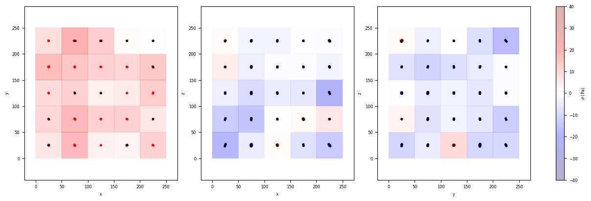
Once again we can represent the obtained stress tensors \(\sigma\) by using the ProjTensor3D function.

ProjTensor3D(Grids_sig,
            CoordGrd_sig,
            SigAVG,
            SigCount,
            scale_factor = 0.1,
            figblocksize=4,
            vmin=-40,
            vmax=40,
            Countmin=5,
            showscale=False,
            nameaxes=['z','y','x'],
            DeviatoricType=1, #<- 1 for dealing with stress: Full stress tensor -> Deviatoric stress tensor
            colorbarlab=r'$\sigma$ (Pa)')

Normal min/max ax0 -0.5432484576144363 20.837223257146253
Normal min/max ax1 -21.085453366830986 6.273667281737579
Normal min/max ax2 -17.612397861857293 9.448668331923121

You have now completed this tutorial. I hope it has been helpfull to you. Go back to FoamQuant - Examples for more examples and tutorials.