Liquid fraction & Bubble radius¶

In this tutorial you will learn to measure liquid fraction and individual bubble radius from respectively phase-segmented (cleaned) and bubble segmented (no-edge) images.

The tutorial is divided in the following sections:

Import libraries
Quantification folders
Get familiar with the input data
Liquid fraction
Get familiar with the input data
Individual bubble properties
Remove bubbles at the edges
Equivalent radius distribution

A) Import libraries¶

[1]:

from FoamQuant import *
import numpy as np
import os
import matplotlib.pyplot as plt; plt.rc('font', size=20)
from tifffile import imread
import pickle as pkl
import pandas as pd

B) Quantification folders¶

[2]:

# Processing folders names
Quant_Folder = ['Q1_LiqFrac_Glob','Q2_LiqFrac_Cartesian','Q3_Bubble_Prop']

# Create the quantification folders (where we are going to save our results)
for Pi in Quant_Folder:
    if  os.path.exists(Pi):
        print('path already exist:',Pi)
    else:
        print('Created folder:',Pi)
        os.mkdir(Pi)

path already exist: Q1_LiqFrac_Glob
path already exist: Q2_LiqFrac_Cartesian
path already exist: Q3_Bubble_Prop

C) Get familiar with the input data¶

[3]:

# Name and directory of the speckle-cleaned images
dircleaned = 'P3_Cleaned/'
namecleaned = 'Cleaned_'

# Read the first image of the series
str_index = strindex(1, n0=3)
print('The string index suffix: ', str_index)
fullname = dircleaned+namecleaned+str_index+'.tiff'
print('The full directory+name: ', fullname)

FirstCleanIm = imread(fullname)

The string index suffix:  001
The full directory+name:  P3_Cleaned/Cleaned_001.tiff

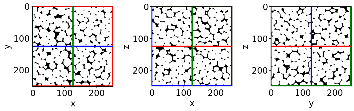
[4]:

# Show a 3D-cut view of the volume
Cut3D(FirstCleanIm,
      showcuts=True, # Shows the red, blue and green cuts.
      nameaxes=['z','y','x'], # Shows the name of the axes, here z,y,x.
      figblocksize=4,# This parrameter gives the size of the produced figure (here 4*3 along the horizontal,  along the vertical).
      cmap='gray')   # The default colormap used by this function is 'gray' but can be modified here.

/gpfs/offline1/staff/tomograms/users/flosch/Rheometer_Jupyter/Jupy_FoamQuant/FoamQuant/Figure.py:90: UserWarning: The figure layout has changed to tight
  plt.tight_layout()

_images/Jupy_FoamQuant_lf_radius_7_1.png

D) Liquid fraction¶

The liquid fraction is an essential parrameter when studying liquid foam. It is quantified from the phase-segmented images, as the number of liquid phase voxels divided by the total number of voxels inside a given volume:

\(\phi_\ell = \frac{N_l}{N_l+N_g}\)

where \(N_l\) and \(N_g\) are the liquid and gas volumes respectively in number of voxels.

Full-image liquid fraction

Here we want to know how the full image liquid fraction evolves with time.

[5]:

# Name and directory where we are going to save the global liquid fractions
dir_lf_glob = 'Q1_LiqFrac_Glob/'
name_lf_glob = 'LiqFrac_Glob_'

# Indexes of the images of our time-series (we are working here with 10 subsequent images of the same foam sample, evolving over time).
imrange = [1,2,3,4,5,6,7,8,9,10]

# Liquid fraction function
LiqFrac_Batch(namecleaned,
              name_lf_glob,
              dircleaned,
              dir_lf_glob,
              imrange,
              TypeGrid='Global', # <- a single value per image
              verbose=True,
              Masktype = [False, False])

Path exist: True
LiqFrac_Glob_001: done
LiqFrac_Glob_002: done
LiqFrac_Glob_003: done
LiqFrac_Glob_004: done
LiqFrac_Glob_005: done
LiqFrac_Glob_006: done
LiqFrac_Glob_007: done
LiqFrac_Glob_008: done
LiqFrac_Glob_009: done
LiqFrac_Glob_010: done

[6]:

# Read the global liquid fractions
List_lf_Global = []
for timei in imrange:
    with open(dir_lf_glob + name_lf_glob + strindex(timei, n0=3) + '.pkl','rb') as file:
        lf_Global = pkl.load(file)['lf']
        List_lf_Global.append(lf_Global)

print('Global liquid fraction as a function of time:\n', np.asarray(List_lf_Global))

Global liquid fraction as a function of time:
 [0.14812106 0.14536508 0.14993783 0.14911722 0.14338045 0.14822921
 0.14275831 0.14482527 0.14253219 0.14275472]

Liquid fraction along a cartesian grid

Now we want to know how the liquid fraction is distributed in space. We are going to use the same function but indicate that we want a cartesian mesh output TypeGrid=’CartesMesh’.

[7]:

# Name and directory where we are going to save the cartesian-grid liquid fractions
dir_lf_car = 'Q2_LiqFrac_Cartesian/'
name_lf_car = 'LiqFrac_Cartesian_'

# Get liquid fraction in cartesian subvolumes
# (volume percentage of liquid in each subvolumes)
LiqFrac_Batch(namecleaned,
              name_lf_car,
              dircleaned,
              dir_lf_car,
              imrange,
              TypeGrid='CartesMesh', # <- a cartesian grid of liquid fractions
              Nz=5,                  # Indicates the number of boxes along z
              Ny=12,                 # ...along y
              Nx=8,                  # ...along x
              verbose=1,
              structured=True,
              Masktype = [False, False]) # <- can be turned on for cylindrical masking around the axis of rotation and in the perriphery

Path exist: True
LiqFrac_Cartesian_001: done
LiqFrac_Cartesian_002: done
LiqFrac_Cartesian_003: done
LiqFrac_Cartesian_004: done
LiqFrac_Cartesian_005: done
LiqFrac_Cartesian_006: done
LiqFrac_Cartesian_007: done
LiqFrac_Cartesian_008: done
LiqFrac_Cartesian_009: done
LiqFrac_Cartesian_010: done

[8]:

# Read all the Cartesian mesh liquid fractions
List_lf_Car = []
for timei in imrange:
    with open(dir_lf_car + name_lf_car + strindex(timei, n0=3) + '.pkl','rb') as file:
        lf_Car = pkl.load(file)['lf']
        List_lf_Car.append(lf_Car)

[9]:

# Result shape: Number of images / Nz / Ny / Nx
np.shape(List_lf_Car)

[9]:

(10, 5, 12, 8)

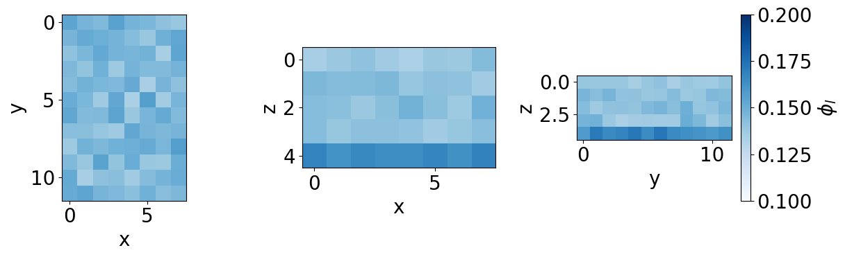
We now gonna represent the liquid fraction field with the same figure tool that we used for observing our images: Cut3D.

[10]:

# Orthogonal cut view of the liquid fraction field obtained from the first image of the series
fig,ax,neg = Cut3D(List_lf_Car[0],
                   nameaxes=['z','y','x'],
                   cmap='Blues',
                   vmin=0.10,
                   vmax=0.20,
                   returnfig=True,
                   figblocksize=4)
fig.colorbar(neg[2], label=r'$\phi_l$')

vmin = 0.1 vmax = 0.2

[10]:

<matplotlib.colorbar.Colorbar at 0x150ffc04b440>

_images/Jupy_FoamQuant_lf_radius_16_2.png

The orthogonal cuts can be seen with Cut3D. The orthogonal projection view can be seen with Proj3D. The projections are averages.

[11]:

# Orthogonal projection view of the time-averaged liquid fraction field
lf_time_average = np.mean(List_lf_Car,0)
fig,ax,neg = Proj3D(lf_time_average,
                    nameaxes=['z','y','x'],
                    cmap='Blues',
                    vmin=0.10,
                    vmax=0.20,
                    returnfig=True,
                    figblocksize=4)
fig.colorbar(neg[2], label=r'$\phi_l$')

vmin = 0.1 vmax = 0.2

/gpfs/offline1/staff/tomograms/users/flosch/Rheometer_Jupyter/Jupy_FoamQuant/FoamQuant/Figure.py:160: UserWarning: The figure layout has changed to tight
  plt.tight_layout()

[11]:

<matplotlib.colorbar.Colorbar at 0x150ff7b98e00>

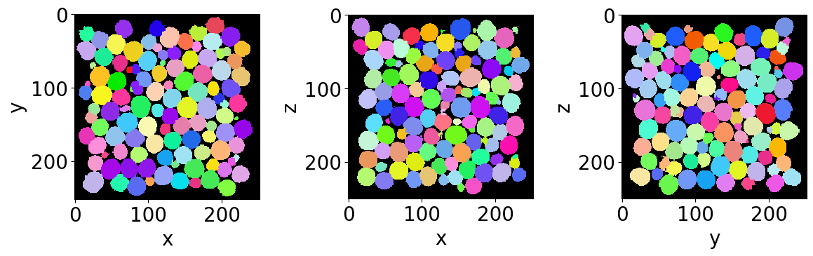
_images/Jupy_FoamQuant_lf_radius_18_3.png

E) Get familiar with the input data¶

Let’s read the first bubble-segmented image of the series (with no bubble on the edges).

[12]:

# Name and directory where the bubble segmented images are saved
dirnoedge = 'P5_BubbleNoEdge/'
namenoedge = 'BubbleNoEdge_'

# Read the first image of the series
Lab = imread(dirnoedge+namenoedge+strindex(1, 3)+'.tiff')

# Since we are now looking at more bubbles let's create a "larger" random colormap: here 500 random colors
rcmap = RandomCmap(500, verbose=False)

# Show a 3D-cut view of the volume
Cut3D(Lab,
      nameaxes=['z','y','x'],
      cmap=rcmap,
      interpolation='nearest',
      figblocksize=4)

_images/Jupy_FoamQuant_lf_radius_21_0.png

F) Individual bubble properties (RegProps)¶

We want here to extract from each bubble region, its equivalent radius. To do so we are going to use the RegionProp_Batch function. It is essentially a wrapped of regionprops from scikit-image.

[13]:

# Name and directory where we are going to save the bubble region properties
dir_Bubble_prop = 'Q3_Bubble_Prop/'
name_Bubble_prop = 'Bubble_Prop_'

RegionProp_Batch(namenoedge,
                 name_Bubble_prop,
                 dirnoedge,
                 dir_Bubble_prop,
                 imrange,
                 verbose=True,
                 endread='.tiff',
                 endsave='.tsv')

Path exist: True
Bubble_Prop_001: done
Bubble_Prop_002: done
Bubble_Prop_003: done
Bubble_Prop_004: done
Bubble_Prop_005: done
Bubble_Prop_006: done
Bubble_Prop_007: done
Bubble_Prop_008: done
Bubble_Prop_009: done
Bubble_Prop_010: done

G) Equivalent radius¶

Let’s open the first saved bubble-properties table with pandas.

[14]:

df = pd.read_csv(dir_Bubble_prop+name_Bubble_prop+strindex(1,n0=3)+'.tsv',sep = '\t')
display(df)

	lab	z	y	x	vol	rad	area	sph	volfit	S1	...	e2y	e2x	e3z	e3y	e3x	U1	U2	U3	U	type
0	1	15.286670	79.575571	183.687352	7622.0	12.208438	1889.990904	0.997457	7696.702997	11.356878	...	12.123131	0.558382	-0.565461	0.558382	12.288122	-0.075555	0.016856	0.058699	0.118985	1
1	2	16.593385	130.636373	17.162980	9584.0	13.177087	2204.247246	0.996115	9674.503042	12.035502	...	12.727413	-0.753596	-0.022763	-0.753596	12.968875	-0.093752	0.022430	0.071322	0.146864	1
2	3	15.635897	172.321484	101.120593	10324.0	13.507857	2309.744140	0.997574	10400.092065	12.805426	...	13.886619	-0.036291	-0.224959	-0.036291	13.241960	-0.055850	-0.019896	0.075747	0.117809	-1
3	4	15.538057	175.370390	217.745069	9328.0	13.058701	2154.914928	0.997516	9371.282698	12.381921	...	12.635434	-0.351062	0.549606	-0.351062	12.901907	-0.054760	-0.022566	0.077326	0.119294	-1
4	5	15.121800	200.194312	163.705468	10936.0	13.769663	2403.553261	0.997433	11037.743266	13.050254	...	14.409886	0.621144	-0.254747	0.621144	13.336950	-0.056747	-0.021472	0.078219	0.121240	-1
...	...	...	...	...	...	...	...	...	...	...	...	...	...	...	...	...	...	...	...	...	...
936	937	232.931714	209.884521	86.382444	9387.0	13.086175	2168.907873	0.998400	9475.291923	12.489027	...	13.894511	-0.170001	-0.174207	-0.170001	12.962521	-0.049827	-0.009192	0.059018	0.095265	-1
937	938	234.656031	34.253836	50.915761	9841.0	13.293833	2235.291662	0.997166	9895.232739	12.680207	...	12.997291	-0.130880	-0.529484	-0.130880	12.878073	-0.049090	-0.035787	0.084877	0.127836	-1
938	939	234.123875	156.617150	218.298716	9889.0	13.315411	2238.448309	0.998684	9938.866176	12.619337	...	13.528568	-0.152264	0.059711	-0.152264	13.724473	-0.055368	0.015737	0.039632	0.085592	1
939	940	234.464956	224.364352	219.393250	9274.0	13.033453	2143.488520	0.998308	9307.919924	12.256650	...	12.866831	-0.005062	0.036705	-0.005062	13.650618	-0.062668	0.017493	0.045175	0.097010	1
940	941	234.799707	24.502990	72.834127	8193.0	12.505991	1977.594288	0.999019	8257.341727	11.949345	...	12.912100	0.136215	0.314278	0.136215	12.591211	-0.048139	0.014913	0.033226	0.073929	1

941 rows × 26 columns

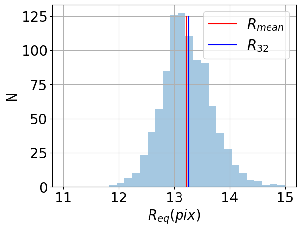
Now we can plot, for example, the bubble equivalent radius distribution, the mean radius and Sauter radius.

[33]:

# Equivalent radius distribution
df['rad'].hist(bins=np.linspace(11,15,30), alpha=0.4)

#Mean radius
Rmean = np.mean(df['rad'])
plt.plot([Rmean,Rmean],[0,125],'r-', label=r'$R_{mean}$')
#Mean Sauter radius
R32 = np.sum(np.power(df['rad'],3))/np.sum(np.power(df['rad'],2))
plt.plot([R32,R32],[0,125],'b-', label=r'$R_{32}$')

plt.xlabel(r'$R_{eq} (pix)$')
plt.ylabel('N')
plt.legend()

[33]:

<matplotlib.legend.Legend at 0x150ff33e2ed0>

_images/Jupy_FoamQuant_lf_radius_27_1.png

You have now completed this tutorial. I hope it has been helpfull to you. Go back to FoamQuant - Examples for more examples and tutorials.